This has probably happened to everyone, and to some people quite often. You receive a meeting invitation from your manager, but it conflicts with a meeting you already have with a colleague. So you try to move that meeting, but the colleague finds that your new proposal now conflicts with another meeting, meaning one of those meetings would need to move too. Finding an optimal schedule for meetings so that no conflicts remain is a very hard problem. Can a quantum computer help?
Background
A few years ago, I started looking into the field of quantum computing. Everywhere I heard that quantum computing was more powerful at solving hard problems, but no one explained what kind of problems. That is what I wanted to learn, so I picked up what some people call the bible of quantum computing, the Quantum Computation and Quantum Information book. The book presents two interesting results in quantum computing. The first is Shor's algorithm, or more generally, the Quantum Fourier Transform. This approach can solve the Hidden Subgroup Problem in polynomial time — in other words, problems where the solution space is periodic. The other highlighted achievement was Grover's algorithm, which provides a quadratic speedup for searching through any NP-hard problem's solution space.
After reading the book, I became interested in more than just the simple question of "What kind of problems can quantum computing solve efficiently?" I wanted to get some hands-on experience and try some quantum computing frameworks, so I started thinking about a good problem to practice on. Most of the NP-hard problems I could think of were optimization problems.
An optimization problem does not search for just any solution, but for the best solution — for example, "What is the shortest path from A to B?" Formally, an optimization problem defines a function \(f: X \rightarrow R\) that assigns a number to every solution; this function is usually called the cost function. The problem is then to find the \(x\) with the minimum value of \(f(x)\). It is also possible to search for the maximum value by simply defining the cost function as \(g(x) = -f(x)\).
Then I realized that the book did not mention optimization problems at all, so I looked into whether there were any quantum computing achievements for optimization problems. I found the breakthrough paper A Quantum Approximate Optimization Algorithm. This paper was published in 2014, so its results could not have been included in a book published in 2010.
Problem
Let's formalize the meeting scheduling problem. The input is a set of unscheduled meetings. Each meeting has a list of required attendees. For simplicity, let's say each meeting requires one hour. The output is a schedule — a time slot assigned to each meeting — such that any two meetings with at least one common attendee are assigned different time slots. The goal is to minimize the number of time slots occupied by all meetings.
For example, consider the following meetings:
| Meeting | Attendees |
|---|---|
| Quantum Mechanics symposium | Albert Einstein, Boris Podolsky, Claude Shannon, John von Neumann |
| Calculus and Differential Equations lecture | Isaac Newton, Gottfried Wilhelm Leibniz, Leonhard Euler |
| Graph Theory and Combinatorics colloquium | Paul Erdős, Leonhard Euler, Frank Ramsey |
| Information Theory symposium | Claude Shannon, Alan Turing, John von Neumann |
The Quantum Mechanics symposium and the Information Theory symposium cannot be scheduled at the same time because Claude Shannon and John von Neumann attend both. The Calculus and Differential Equations lecture and the Graph Theory and Combinatorics colloquium cannot overlap because Leonhard Euler attends both.
One optimal schedule is:
| Time | Meeting |
|---|---|
| 8:00 | Quantum Mechanics symposium |
| 8:00 | Calculus and Differential Equations lecture |
| 9:00 | Graph Theory and Combinatorics colloquium |
| 9:00 | Information Theory symposium |
Minimum Graph Coloring
The scheduling problem can be transformed into the Minimum Graph Coloring problem.
Graph coloring is the task of assigning a color to each vertex such that no two vertices connected by an edge share the same color. The minimum graph coloring problem asks: what is the smallest number of colors needed to accomplish this? That number is called the chromatic number of the graph.
Transforming the schedule into a graph
The scheduling problem maps to a graph in two steps:
- Each meeting becomes a vertex.
- Two vertices are connected by an edge if and only if the two meetings share at least one attendee.
Applying this to our example produces the following graph:
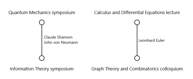
We then find a coloring of this graph using the minimum number of colors. Each color is assigned a unique time slot. It is straightforward to see why this works: if two conflicting meetings were assigned the same time slot, they would be connected by an edge yet share the same color — which violates the coloring constraint. Therefore, a valid coloring guarantees a conflict-free schedule, and minimizing the number of colors minimizes the number of time slots.
Quantum Approximate Optimization Algorithm for Minimum Graph Coloring
Now we arrive at the quantum part. The Quantum Approximate Optimization Algorithm (QAOA) is a hybrid quantum-classical algorithm designed to solve combinatorial optimization problems. "Hybrid" means it uses a quantum computer and a classical computer together, playing to the strengths of each.
Before QAOA can run on a quantum computer, the solution space of the optimization problem must be encoded in quantum states. The usual form of encoding is a binary encoding into multiple qubits in basis \(|0 \rangle\) and \(|1 \rangle\), similar to how the solution would be encoded in a classical binary array. In context of the Minimum Graph Coloring problem, this means that every vertex coloring must be assigned to a unique quantum state (or classical binary string). Then the optimization cost function is defined as a cost Hamiltonian \(H_c\). A "Hamiltonian" is an operator or function that calculates the total energy of the quantum state. In this way, an optimization problem of finding the best solution can be transformed into the problem of finding a quantum state with the lowest energy.
There are many ways to look at how QAOA works, and I found an interesting one in An Introduction to the Quantum Approximate Optimization Algorithm. The paper mentions the Adiabatic Theorem and its implication, stating:
If a quantum system is in the lowest energy state of the initial Hamiltonian \(H_i\) and it is slowly transformed to the final Hamiltonian \(H_f\), then the system stays in the lowest energy state through the transformation, ending in the lowest energy state of Hamiltonian \(H_f\).
So a quantum optimization algorithm would start with a well-known initial Hamiltonian and its well-known lowest energy state. For an \(n\)-qubit system, a good starting point is the Hamiltonian
where \(X_i\) is the Pauli-X matrix applied to qubit \(i\). It is easy to check that the lowest energy state of \(H_i\) is the superposition of all basis states.
Then we define a time-evolving Hamiltonian for the system that would slowly transform from \(H_i\) to \(H_f\). So the Hamiltonian at time \(t\) would be
This means that the quantum circuit for the full time evolution would need to implement the unitary operation
Unfortunately, in general this quantum circuit would need an infinite number of gates to implement this operation precisely. However, it is possible to approximate it by splitting the continuous time interval \(t \in [0, 1]\) into a finite number of steps. The steps do not have to be the same size, so the circuit would be the product of the following unitary operations.
where \(t_k\) are timestamps on the interval \([0, 1]\). We can generalize this operation by replacing \((1-t_k)\) with \(\beta_k / 2\) and \(t_k\) with \(\gamma_k / 2\). Then the operation looks like
A nice property of this operation is that, for a well-chosen Hamiltonian, the operation \(e^{-i \frac{\alpha}{2} H}\) is easy to implement in a quantum circuit. Usually it just needs to entangle specific qubits and then simply rotate a specific qubit by angle \(\alpha\). Also, increasing the number of steps in the circuit improves the precision of the calculation, as
Another way to look at it is that the algorithm starts with a superposition of all possible states and then iteratively alternates between the final and initial (also known as the mixer) Hamiltonians, with different weights / rotation angles. The final Hamiltonian shifts the phase toward optimal solutions, thus amplifying optimal solutions and suppressing bad ones. The mixer Hamiltonian then mixes the state so that the algorithm does not get stuck in a local minimum, but instead searches for the global one.
Final Hamiltonian
Now that we know how the quantum optimization algorithm works, we need to find the final Hamiltonian and the angles \(\beta_i\) and \(\gamma_i\).
Recently, a new study proposed a qubit-efficient cost Hamiltonian for the Minimum Graph Coloring problem. It was published in "Qubit-efficient and gate-efficient encodings of graph partitioning problems for quantum optimization". It suggests encoding the coloring in the following way.
Each vertex (meeting) is assigned a block of \(L = \lceil \log_2 C \rceil\) qubits, where \(C\) is an upper bound on the chromatic number derived from Brooks' theorem. These \(L\) qubits encode the vertex's color as a binary integer. With \(n\) vertices, the coloring register uses \(n \cdot L\) qubits total.
For example, with 4 meetings and a chromatic number bound of 3, the number of bits per meeting is \(L = \lceil \log_2 3 \rceil = 2\), which leads to 8 qubits total in the coloring register.
The paper phrases the cost function directly in terms of classical bits, before any quantum encoding enters the picture. Let \(x_{v,k} \in \{0, 1\}\) denote bit \(k\) of vertex \(v\)'s color, so that vertex \(v\)'s color is the integer \(\sum_{k} x_{v,k} 2^k\). The cost function — called a Hamiltonian by analogy with its quantum counterpart — is
The first term is the adjacency penalty. The factor \(2x_ux_v - x_u - x_v + 1\) is just the XNOR of the two bits written as a polynomial: it equals \(1\) when \(x_u = x_v\) and \(0\) otherwise. So the product over all \(L\) bits of an edge \((u, v)\) evaluates to \(1\) exactly when every bit matches — that is, when the two meetings have been assigned the same color — and to \(0\) the moment a single bit differs. Summed over all edges and scaled by a constant \(A\), this term adds energy \(A\) for every conflicting pair of meetings and zero energy for every properly colored edge.
The second term is the lexicographic penalty. Taken alone, the adjacency term is satisfied by any proper coloring, including wasteful ones — nothing stops the optimizer from giving every meeting its own color. The weights \(P_k\) grow with \(k\) fast enough that setting a higher-order color bit always costs more than a lower-order one, which nudges the optimizer toward colorings that only use the lower-order bits, i.e. the smallest color indices. This is exactly the minimum coloring we are after. In the paper, \(A = (n+1)^L\) and \(P_k = (n+1)^k\), where \(n\) is the number of vertices; both are chosen large enough that satisfying adjacency is always prioritized over lexicographic minimization, but small enough that lexicographic terms converge sufficently for approximation.
To run this Hamiltonian on a quantum computer, it needs to be expressed as an operator acting on qubits, and the natural choice for encoding a single bit is the Pauli-\(Z\) operator, whose eigenvalues are \(+1\) and \(-1\) rather than \(0\) and \(1\). The standard substitution is
so \(Z_{v,k} = +1\) when bit \(k\) of vertex \(v\)'s color is \(0\), and \(Z_{v,k} = -1\) when it is \(1\). Plugging this into the adjacency factor collapses it to
Taking the product of this over all \(L\) bits and expanding it turns the single XNOR factor into a sum over every non-empty subset \(S\) of bit positions, since \(\prod_k (1 + Z_{u,k}Z_{v,k})/2 = 2^{-L}\sum_{S \subseteq \{ 0, \ldots, L-1 \}} \prod_{k \in S} Z_{u,k}Z_{v,k}\) (the \(S = \emptyset\) term contributes only a constant). That factor of \(2^{-L}\) combines with the classical-level coefficient \(A = (n+1)^L\) to give a smaller effective weight, \((n+1)^L \cdot 2^{-L} = \left(\frac{n+1}{2}\right)^L\), on each qubit-level term. After dropping the remaining constant terms — they shift every state's energy equally and therefore never change which state has the lowest energy — the cost Hamiltonian becomes
with \(A' = \left(\frac{n+1}{2}\right)^L\) — the rescaled, qubit-level version of the classical-level \(A\) from before.
Implementation
Now that we know theoretically how the quantum circuit should look, let's implement it. The first step for me was to look at which quantum computing framework I would like to use. My goal was to learn, not necessarily to run the program on an actual quantum computer, so my preference was a vendor-independent framework. Therefore, I tried to avoid Qiskit or Q#, even though there were a lot of references to Qiskit. I found a possibly interesting project, ProjectQ. Unfortunately, just installing it produced a warning that it was not compatible with the new version of Python 3.14, and even running a simple example didn't work on this version. Then I noticed that the latest release was from 2022, so I decided to try something else.
The next candidate was PennyLane, which worked very well, so the implementation in this post uses this framework.
Initial Hamiltonian implementation
Let's start with the function that implements the initial Hamiltonian.
def _get_initial_hamiltonian(self, qubit_count: int) -> qpl.Hamiltonian:
    coeffs = [1.0] * qubit_count
    ops = [1.0 * qpl.PauliX(i) for i in range(qubit_count)]
    return qpl.Hamiltonian(coeffs, ops)
PennyLane represents a Hamiltonian as a weighted sum of operators: a list of coefficients paired with a matching list of operators. Here every coefficient is \(1.0\) and every operator is \(X_i\) for qubit \(i\), which gives \(H_i = \sum_i X_i\) — the transverse-field mixer from the theory section, applied across all qubit_count qubits.
One detail worth flagging: the sign here is the opposite of the \(-\sum_i X_i\) used earlier. This does not matter in practice. The mixer only ever appears inside qpl.qaoa.mixer_layer as \(e^{-i\beta H_i}\), so flipping the sign of \(H_i\) is equivalent to negating \(\beta\), and the classical optimizer is free to pick whichever sign works best within its bounds.
Final Hamiltonian implementation
def _get_final_hamiltonian(self) -> qpl.Hamiltonian:
    n = self.vertex_count
    num_bits = self.color_bits_count

    def qubit(vertex_idx: int, bit: int) -> int:
        return vertex_idx * num_bits + bit

    coeffs: list[float] = []
    ops: list[qpl.operation.Operator] = []

    # --- Adjacency term ---
    adj_coeff = ((n + 1) / 2) ** num_bits
    for u, v in self.graph.edges():
        ui = self.vertices.index(u)
        vi = self.vertices.index(v)
        for mask in range(1 << num_bits):
            subset_qubits: list[int] = []
            for k in range(num_bits):
                if mask & (1 << k):
                    subset_qubits.append(qubit(ui, k))
                    subset_qubits.append(qubit(vi, k))

            if subset_qubits:
                op: qpl.operation.Operator = qpl.PauliZ(subset_qubits[0])
                for q in subset_qubits[1:]:
                    op = op @ qpl.PauliZ(q)

                coeffs.append(adj_coeff)
                ops.append(op)

    # --- Lexicographic term ---
    for k in range(num_bits):
        coeff = -0.5 * (n + 1) ** k
        for i in range(n):
            coeffs.append(coeff)
            ops.append(qpl.PauliZ(qubit(i, k)))

    return qpl.Hamiltonian(coeffs, ops)
This is a direct transcription of the Hamiltonian derived above. Four attributes of the solver instance have impact on the Hamiltonian:
self.graph— the conflict meeting graph itself. Each edge represents a conflict between meetings. The function builds an adjacency term for each edge.self.vertex_count(\(n\)) — the number of meetings, computed once aslen(graph.nodes()). It sets the base of the exponential weights \(A\) and \(P_k\).self.color_bits_count(\(L\)) — the number of qubits used per vertex, computed from the logarithm of the Brooks'-theorem bound described earlier.self.vertices— a fixed-order list of the graph's nodes, used to translate a vertex (which might be an arbitrary Python object, like a meeting name) into an integer index. That index is whatqubit()uses to compute the qubit offset for a given vertex and bit.
The small helper function qubit calculates the index of the qubit that represents a specific bit of the color of a specific vertex. Notice that the color encoding is little-endian: the more significant bit has the higher qubit index.
The nested loop over mask in range(1 << num_bits) is the code's way of iterating over every non-empty subset \(S\) of bit positions: each bit of mask says whether bit position \(k\) belongs to \(S\), and whenever it does, both \(Z_{u,k}\) and \(Z_{v,k}\) are folded into the running tensor product via PennyLane's @ operator (which composes operators into a multi-qubit Pauli string). The lexicographic term above is a much simpler double loop — one term per bit position \(k\) per vertex \(v\), with coefficient \(-\frac{1}{2}(n+1)^k\) exactly as derived above.
Quantum circuit implementation
def get_colors(self, angles: list[float]) -> tuple[list[int], float]:
    @qpl.qnode(self._dev)
    def circuit() -> npt.NDArray[np.int_]:
        self._execute_layers(pnp.array(angles))
        return qpl.probs(wires=range(self.all_qubits_count))

    probabilities = circuit()

    state = np.argmax(probabilities)
    probability = probabilities[state]

    return (self._decode_colors(state), probability)

def _execute_layers(self, angles: npt.NDArray[np.float64]) -> None:
    for i in range(self.all_qubits_count):
        qpl.Hadamard(wires=i)

    half = len(angles) // 2
    for beta, gamma in zip(angles[:half], angles[half:]):
        qpl.qaoa.cost_layer(gamma, self.final_hamiltonian)
        qpl.qaoa.mixer_layer(beta, self.initial_hamiltonian)

def _decode_colors(self, state: np.int_) -> list[int]:
    colors: list[int] = []

    for i in range(self.vertex_count):
        color = 0
        bit_value = 1
        for j in range(self.color_bits_count):
            bit_index = i * self.color_bits_count + j
            # Reflect: qubit 0 is the highest bit of the integer.
            bit_index = self.coloring_qubits_count - 1 - bit_index
            if state & (1 << bit_index):
                color += bit_value
            bit_value <<= 1

        colors.append(color)

    return colors
The get_colors function calculates the coloring with the highest probability. The function uses the following attributes of the solver instance:
self.coloring_qubits_count(\(n \cdot L\)) — the total number of qubits. It equals the number of vertices times the number of coloring bits per vertex.self.all_qubits_count— same ascoloring_qubits_counthere. However, there is a version with some ancilla qubits that would be counted in this attribute too.
If the angles are provided, running the circuit is just a matter of executing it and reading out qpl.probs(), which returns the full probability distribution over all \(2^n\) basis states — the quantum-simulator equivalent of running the real circuit many times and building a histogram of measurement outcomes. np.argmax picks the single most likely basis state, and _decode_colors turns that state back into a coloring. For color decoding, keep in mind that the encoding is little-endian.
The interesting part is _execute_layers, since it is what turns the abstract \(U_p\) formula from the theory section into an actual sequence of gates:
The first loop applies a Hadamard gate to every qubit, which is what actually prepares the uniform superposition \(\psi_0 = |+\rangle^{\otimes n}\). The angles list is the flat \((\beta_0,\ldots, \beta_{p-1}, \gamma_0,\ldots, \gamma_{p-1})\) array provided as parameter, split in half and zipped back into \(p\) (beta, gamma) pairs. Each pair becomes one layer: qpl.qaoa.cost_layer compiles \(e^{-i\gamma H_f}\) into gates directly from the final_hamiltonian object built earlier, and qpl.qaoa.mixer_layer does the same for \(e^{-i\beta H_i}\) using initial_hamiltonian. Stacking \(p\) of these pairs is exactly the product \(U_p\) from the theory section.
Finding angles — optimizing
Now we have the quantum circuit with angles as parameters, so the only question is how to set up those angles. Unfortunately, this is the hardest part of QAOA. The first thing we need is to implement a function that returns the expectation value of the quantum circuit measured using the final Hamiltonian. This means we would not measure all qubits individually, but only the total energy. In other words, if we start with the initial state as a superposition of all basis states
and run the circuit that implements the unitary operation
and we get the final state
then the expectation value of the final Hamiltonian (or mean total energy) is
The following function creates such circuit.
def _build_cost_circuit(self) -> qpl.QNode:
    @qpl.qnode(self._dev)
    def circuit(angles: npt.NDArray[np.float64]) -> float:
        self._execute_layers(angles)
        return qpl.expval(self.final_hamiltonian)

    return circuit
This looks almost identical to the circuit inside get_colors, and it is — same device, same _execute_layers call — but it returns qpl.expval(self.final_hamiltonian) instead of qpl.probs(). Instead of the full probability distribution, qpl.expval returns a single number: \(\langle \psi_f | H_f | \psi_f \rangle\), the expectation value we derived above.
The quantum simulator calculates the exact expectation value. Using a real quantum computer, the function would return the mean measured value over multiple measured samples.
Next we will use classical optimization algorithms to find optimal parameters that minimize the output of the _cost_circuit function. There are many algorithms, and Claude recommended COBYLA (Constrained Optimization BY Linear Approximation) that is implemented in SciPy.
def find_optimal_angles(self) -> list[float]:
    angles: list[float] = []
    angles += [self.starting_beta] * self.evolution_count
    angles += [self.starting_gamma] * self.evolution_count

    bounds: list[tuple[float, float]] = []
    bounds += [(0, math.pi / 2)] * self.evolution_count
    bounds += [(0, math.pi)] * self.evolution_count

    options: dict[str, Any] = { "maxiter": self.optimization_steps }

    def cost_fun(angles: npt.NDArray[np.float64]) -> float:
        return self._cost_circuit(angles)

    result = opt.minimize(
        cost_fun,
        pnp.array(angles),
        method="COBYLA",
        bounds=bounds,
        options=options)

    return [float(x) for x in result.x]
evolution_count is the class variable that sets \(p\), the number of iterations (evolutions) in the QAOA circuit. It also defines the number of \(\beta\) and \(\gamma\) angles. The function creates a list of angles \((\beta_0,\ldots, \beta_{p-1}, \gamma_0,\ldots, \gamma_{p-1})\) and sets each \(\beta_i\) to starting_beta and each \(\gamma_i\) to starting_gamma — the array with the layout that is expected by _execute_layers function. The bounds keep every \(\beta\) in \([0, \pi/2]\) and every \(\gamma\) in \([0, \pi]\), which follows from the periodicity of the rotations each angle controls — searching outside these ranges would just retrace angles already covered inside them.
cost_fun is a thin wrapper around the _cost_circuit QNode built above, and opt.minimize(..., method="COBYLA") hands it to SciPy's COBYLA optimizer, which repeatedly proposes new angle values, evaluates the quantum circuit at each one (via cost_fun), and uses those samples to find the optimal angles. optimization_steps caps how many such evaluations COBYLA is allowed to make. The angles it converges to (result.x) are what gets passed into get_colors afterward.
Putting it all together
All the pieces — Hamiltonians, circuit, optimizer — come together in one function that takes a networkx graph and returns a colored copy of it.
def min_graph_coloring(graph: Graph[Any]) -> GraphColoringResult:
    result = graph.copy()

    # A graph with no vertices or edges needs no quantum computation at all.
    if not graph.nodes():
        return GraphColoringResult(result, 1.0)

    if not graph.edges():
        for v in result.nodes():
            result.nodes[v]["color"] = 0
        return GraphColoringResult(result, 1.0)

    solver = GraphColoringSolver(result)
    optimal_angles = solver.find_optimal_angles()

    probability = 0.0

    if len(optimal_angles) > 0:
        colors, probability = solver.get_colors(optimal_angles)

        # The most probable measurement is not guaranteed to be a valid
        # coloring — verify before accepting it.
        if _verify_coloring(result, solver.vertices, colors):
            for i, v in enumerate(solver.vertices):
                result.nodes[v]["color"] = colors[i]
            return GraphColoringResult(result, probability)

    # Fallback: unique color per vertex (always a valid n-coloring).
    for i, v in enumerate(solver.vertices):
        result.nodes[v]["color"] = i
    return GraphColoringResult(result, probability)
Two edge cases are handled before any quantum computation happens: a graph with no vertices needs nothing, and a graph with vertices but no edges has no conflicts, so every meeting can share color 0. Otherwise a GraphColoringSolver is built for the graph — this is the constructor that computes the Brooks'-theorem bound, lays out the qubits, and builds initial_hamiltonian and final_hamiltonian — angles are optimized with find_optimal_angles, and the resulting state is decoded with get_colors.
That last step is a heuristic, not a guarantee: QAOA can converge on a state that is not a valid coloring at all, so _verify_coloring double-checks the decoded colors against the actual graph before accepting them. If verification fails — or if the optimizer returned no angles at all — the function falls back to assigning every vertex its own color, which is trivially a valid coloring, but likely far from minimal.
Full source code can be found at https://github.com/duracellko/qcalendar.
Tuning
The code above has three variables whose setup I have not yet mentioned: starting_beta, starting_gamma, and evolution_count. These need to be tuned by experimentation.
I ran some configurations on a quantum simulator. First, I started with a graph with 4 vertices and 2 edges.
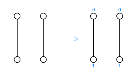
The upper bound on the chromatic number of this graph is 2, so the algorithm needs only 4 qubits to run.
The following variables were set:
evolution_count: 2maxiter(COBYLA - maximum number of evaluations): 100
The following table presents the probability results for different values of starting_beta and starting_gamma.
| \(\beta\) | \(\gamma\) | Probability | All solutions probability |
|---|---|---|---|
| 0.001 | 0.001 | 0.227535758 | 0.910143032 |
| 0.01 | 0.01 | 0.227534724 | 0.910138897 |
| 0.1 | 0.1 | 0.227536269 | 0.910145077 |
| \(\pi / 4\) | \(\pi / 4\) | 0.249993679 | 0.999974715 |
| \(\pi / 8\) | \(\pi / 4\) | 0.249981939 | 0.999927754 |
| \(\pi / 8 + 0.01\) | \(\pi / 4 + 0.01\) | 0.235672315 | 0.94268926 |
- Probability - probability of the resulting coloring with the highest probability.
- All solutions probability - sum of probabilities of all colorings with the minimum number of colors. This is the probability of the optimal outcome. Keep in mind that there is more than 1 optimal solution.
Then I ran the program on the graph with 4 vertices and 4 edges.
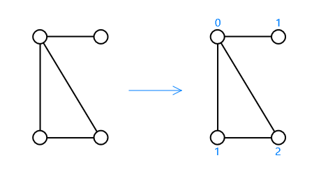
The upper bound on the chromatic number of this graph is 3, so the algorithm needs 8 qubits to run. The same values were used for evolution_count and maxiter.
The following table presents the probability results for different values of starting_beta and starting_gamma.
| \(\beta\) | \(\gamma\) | Probability | All solutions probability |
|---|---|---|---|
| 0.001 | 0.001 | 0.019252569 | 0.054215138 |
| 0.01 | 0.01 | 0.013778213 | 0.100561002 |
| 0.1 | 0.1 | 0.017372671 | 0.047633037 |
| \(\pi / 4\) | \(\pi / 4\) | 0.00390625 | 0.046875 |
| \(\pi / 8\) | \(\pi / 4\) | 0.023170804 | 0.165677839 |
| \(\pi / 8 + 0.01\) | \(\pi / 4 + 0.01\) | 0.026776257 | 0.125146567 |
It seems that a good starting point would be somewhere around \(\pi / 8\) and \(\pi / 4\). However, this is based only on simulation.
Summary
We mapped meeting scheduling to the minimum graph coloring problem and showed how QAOA can be used in a hybrid quantum-classical workflow to search for good schedules. Then we implemented the QAOA algorithm using PennyLane. The implementation includes the initial and final Hamiltonians, the quantum circuit, and the classical optimizer. Finally, we ran some experiments on a quantum simulator to find good starting values for the angles.
Note: Full source code can be found at https://github.com/duracellko/qcalendar.